

Technical Dispatches, as related by the minds behind Karman+, are intended to bring readers behind the scenes and into the research. In this edition, Dr. Lauri Siltala, a Finnish astronomer and asteroid characterization specialist at Karman+, details how Karman+ works to stay ahead of the curve… analysis.
Karman+ is targeting carbonaceous asteroids as a source for useful resources to utilize in the space economy, including water. In fact, the presence of water is a key indicator that the asteroid is the type of object we’re interested in. Naturally, it follows that we must target and identify near-Earth asteroids likely to contain water. In practice, the standard approach to water detection is through spectroscopy. There exist several well-known spectral features around 3 µm that point to the presence of water, ideally in combination with another spectral feature around 700 nm. These are demonstrated by the below figure of Rivkin & DeMeo, 2019:
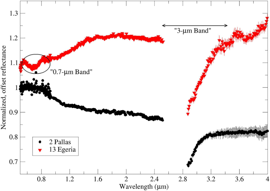
As is often the case with astronomical observations, the atmosphere proves to be a significant challenge in such efforts in that it contains water itself and therefore unavoidably blocks a significant amount of infrared radiation around 3 µm. That does not make this band impossible to observe from Earth, but there are few telescopes that are capable of doing so. Space telescopes, of course, do not have to worry about the atmosphere, but there are very few of those.
Asteroids are abundant, but not created equal
In the absence of direct observations, we may have to rely on the fact that carbonaceous asteroids in general are thought to be among the most water rich asteroids. While there certainly is expected to be variation between the water content of individual carbonaceous asteroids, modern planetary science implies that we will be likely to find water no matter which carbonaceous asteroid we visit. One caveat to this is that some near-Earth asteroids, or NEAs, get very close to the Sun, where the heat will cause water to sublimate (transition from solid to gas state) and thus deplete the water content of such asteroids. Clearly, we would not want to go to such an asteroid. Fortunately, there exists a probabilistic model for estimating the near-Sun dwell times of individual asteroids based on their orbital parameters (Toliou et al. 2021), which we apply to avoid such water-depleted asteroids.
That’s one hurdle solved. However, there is another practical challenge. Carbonaceous asteroids are plentiful in the Solar System and in fact among the most common — so it follows that it is easy to find known carbonaceous NEAs, including some that are known to be hydrated such as 2004 VJ1 (Mahlke et al. 2022), which is relatively accessible for the spacecraft. But, despite their relative abundance, our use case requires observable data that suggests the resources we need to thrive. Naturally, going through the vast effort to reach an asteroid without the yield we need would be a devastating blow to the mission.
As a company, we need to become profitable in order to survive, and to this end, we need asteroids that are even easier to reach with low delta-V requirements than 2004 VJ1 is. Such asteroids do exist, and we have successfully identified them; only, they are all very small and, by extension, difficult to observe. This means that there is a severe lack of observational data with these asteroids, and not a single one is known to be carbonaceous. In an earlier Technical Dispatch we discussed how we leverage existing data to better understand these asteroids and this is yet another aspect of that challenge!
Keying in on carbonaceous from afar
So, how can we figure out which of these asteroids are carbonaceous and which are not, in the absence of actual spectral data? The most straightforward way would be to simply observe them ourselves, but, with a couple of exceptions, this is not feasible as asteroids this dim are not practically observable outside brief observability windows which are few and far between. The only remaining option is to use the data that is available, and the simple fact that these asteroids are known guarantees that someone, somewhere, must have observed each of them in the past. In practice, this data consists of astrometric and photometric measurements, i.e. the asteroid’s position on the sky and its brightness respectively, at some specific point in time.
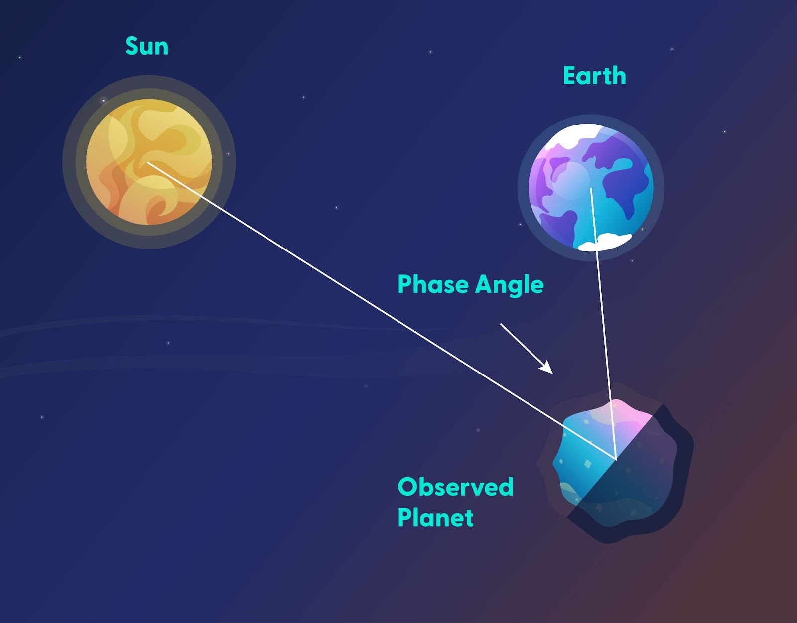
This is where so-called phase curves come in. It is well established that an asteroid’s brightness has, among other things, a dependency on the phase angle, or the angle between the Sun and the observer as seen from the asteroid at the time of observation. Without exception, a larger phase angle means a lower brightness, and a phase curve depicts the relationship between the magnitude, or brightness, of the asteroid and the phase angle, but the shape of this curve differs per asteroid.
There exist a number of different systems for modeling these phase curves for a given asteroid; the currently noteworthy ones are the (H, G1, G2) and (H, G12) systems as first defined by Muinonen et al, 2010. The first author was, incidentally, also one of my PhD thesis advisors. The overall principle is the same; one fits the phase curves, defined as functions of these parameters, into the available photometric observations as a function of the phase angles at the time of observation. The (H, G1, G2) system is theoretically a superior approach but it relies on a large number of quality observations being available, on the order of hundreds, which we often do not have. The (H, G12) function on the other hand, is a simplification of the previous method which does much better when only a small number of observations are available.
With these models, we have parameters for a number of scenarios relative to the data on hand and what we can observe. More progress! But let us take a step back. How does any of this help us figure out which asteroids are carbonaceous and which are not?
Have a look at this table from the work of Oszkiewicz et al, 2012:
| Complex | Nr of objects | Mean | Std |
|---|---|---|---|
| A | 16 | 0.39 | 0.19 |
| C | 391 | 0.64 | 0.16 |
| D | 23 | 0.47 | 0.14 |
| E | 26 | 0.39 | 0.16 |
| O | 3 | 0.57 | 0.05 |
| Q | 72 | 0.41 | 0.14 |
| R | 4 | 0.24 | 0.18 |
| S | 584 | 0.41 | 0.16 |
| V | 35 | 0.41 | 0.14 |
| X | 212 | 0.48 | 0.19 |
From these statistics, it is evident that the distribution of G12 differs per taxonomic complex and the carbonaceous C complex in particular stands out, having a significantly larger mean G12 value than any other complex besides the extremely rare O types. Intuitively, this means that an asteroid with a large G12 value is likely to be carbonaceous, while asteroids with low G12 values likely are not. As data is available, this value is something we can compute. Cool!
Applying the data to our purpose
Here’s where it all comes back to our work at Karman+. Now we have a way to do our own science on asteroids on which no studies have been published. I wrote a Python program, called Phazon, to compute phase functions for arbitrary asteroids. Astronomical surveys are fortunately very good at reporting their observations to the IAU-operated Minor Planet Center, which for our purposes is highly convenient; there is a single repository from which we can download all of the available observations for our asteroids. So, Phazon automatically fetches all of the data available for an arbitrary asteroid and processes and calibrates the data.
What sort of processing is required, you ask? Intuitively, an asteroid’s observed brightness will also depend on its distance from the observer at the time of observation; asteroids that are further away are dimmer. Clearly, we cannot just use the observed brightnesses as is, but they must all be calibrated to correspond to brightness at a single constant distance. When the distance during the observation is known, this is trivial to compute. This distance is not, however, an observed quantity, but a computed one. While we could compute it ourselves without too much effort, it was simpler to use the JPL Horizons system to automatically fetch this quantity for each of our observations together with the phase angle, which is also a computed quantity that we will need later. That is the first step done.
The next thing to note is that photometric observations are practically always conducted with filters which only allow light from specific wavelength bands to reach the detector. The phase function may also look different for different wavelength bands, and an asteroid’s brightness will similarly depend on the filter in use. Thus, it would be ideal to only use observations from a single filter. In practice, we have to be a little more flexible, as many of the asteroids we care about have so little available data that we must use all of it at once. Fortunately, there exist statistical corrections published by the Minor Planet Center for calibrating observations of different bands to the V band, and we apply precisely these corrections to the observations. With this work done, we have everything we need to fit the (H, G12) phase function.
Without getting into the nitty gritty details, let’s take the asteroid 2018 VO9 as an example case. The (H, G12) phase function for this asteroid as computed by Phazon looks like this:
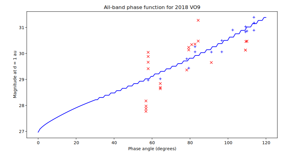
There’s quite a bit of stuff going on in that graph. The blue line is the (H, G12) phase function fitted into the data; its shape is defined by the G12 parameter — and if the jagged look catches your interest, it is due to the lookup tables Phazon currently uses in computing the phase function values. In time, these will be replaced and the function smoothed. The blue and red points represent all of the data that is available for the asteroid, where the red crosses represent data that has been rejected as statistical outliers and excluded from the actual phase function fit due to their apparently high errors. The blue data points, on the other hand, match the phase function well enough.
So what’s the G12 value here, you ask? Phazon says G12 = 0.62 ± 0.18. Looking back at the statistics I shared earlier in Table 1, it sure looks like this asteroid is most likely carbonaceous, does it not? Because of the uncertainties and the width of the G12 distributions for different complexes, we cannot say that 2018 VO9 is carbonaceous for sure based on this result. What we can say is that it is more likely to be carbonaceous than anything else. And make no mistake, that is already a large improvement beyond the initial state, which was “we have no idea about this asteroid’s spectral class.”
There is another little bonus to be had here; readers of the blog may notice that Technical Dispatch #0 already spoke of the H parameter, which is simply the asteroid’s absolute magnitude, a critical parameter for estimating an asteroid’s size. This is exactly how it is determined, but databases such as the JPL’s Small-Body Database (SBDB) usually estimate it by assuming a constant value for the slope parameter G. Phazon does not; therefore the H values it finds are more realistic and thus this work also leads to improved size estimates for our target asteroids. It is far from a night-and-day difference, but all these improvements add up.
Phazon and beyond
So what’s next for Phazon? Enlightened readers may have noticed that I have neglected something in the above. Asteroids spin and are generally not spherically shaped; these things, too, affect the observed brightness. The larger the area of the asteroid facing the observer is, the brighter the asteroid will seem. What’s more, spin and shape will make this quantity not constant.
When the spin and shape are known, it is straightforward to remove these effects from the data, but for most asteroids they are not, and the lack of this correction may, in part, explain the large spread of the observed data points we see in the figure. Perhaps we can estimate these from this data ourselves and learn even more of these asteroids while improving the phase function fits in the process. This too is traditionally done with photometry, only with a much higher temporal resolution than what we have to work with. There is another possibility here too; comparing an asteroid’s brightness at different wavelength bands — the asteroid’s color, in a sense as this, too, depends on the spectral class. I’ll just have to try and see what comes of it all… perhaps you’ll read about it in a future Technical Dispatch!
References
- M. Mahlke, B. Carry and P. A. Mattei. (2022). Asteroid taxonomy from cluster analysis of spectrometry and albedo. Astronomy & Astrophysics, Volume 665, A26.
- K. Muinonen, I. Belskaya, A. Cellino, M. Delbò, A-C. Levasseur-Regourd, A. Penttilä and E. Tedesco. (2010). A three-parameter magnitude phase function for asteroids. Icarus, Volume 209, Issue 2, pp. 542-555.
- D. Oszkiewicz, E. Bowell, L. Wasserman, K. Muinonen, A. Penttilä, T. Pieniluoma, D. Trilling and A. Rivkin & F. DeMeo. (2010). How Many Hydrated NEOs Are There?., The Journal of Geophysical Research: Planets, Volume 124, Issue 1, pp. 128-142
- C. Thomas. (2012). Asteroid taxonomic signatures from photometric phase curves. Icarus, Volume 219, Issue 1, pp. 283-296.
- A. Toliou, M. Granvik and G. Tsirvoulis. (2021). Minimum perihelion distances and associated dwell times for near-Earth asteroids. Monthly Notices of the Royal Astronomical Society, Volume 506, Issue 3, pp.3301-3312.